Research

FEniCS project

The FEniCS project comprises a number of libraries as a general toolbox for the computation of the finite element discretisation of partial differential euqations. For example, consider a standard linear finite element formulation which reads: find \(u_h \in V^h\) such that

\[a(u_h, v) = l(v) \quad \forall v \in V^h,\]

where \(u_h\) and \(v\) are the trial and test functions, respectively, belonging to the finite element space of functions \(V^h\). In the context of the Poisson problem in a domain \(\Omega\), the bilinear and linear formulations \(a(\cdot,\cdot)\) and \(l(\cdot)\) are given by

\[\begin{aligned} a(u, v) &= \int_\Omega \nabla u \cdot \nabla v \; \mathrm{d} x, \\ l(v) &= \int_\Omega f \; v \; \mathrm{d} x. \end{aligned}\]

Using FEniCS the finite element space \(V^h\) is constructed by Basix. The finite element formulation is represented in python by exploiting symbolic algebra as implemented in the unified form language (UFL)

a = ufl.inner(ufl.grad(u), ufl.grad(v)) * ufl.dx
l = ufl.inner(f, v) * ufl.dx

This symbolic representation is then automatically translated to a C code implementation of the local element kernel by the FEniCSx form compiler (FFCx)

Click to expand FFCx generated C code of the bilinear formulation

void tabulate_tensor_integral_c2833a6d26cdde02c09f8cbb4b3bf92016ec9e7e(double* restrict A,
                                    const double* restrict w,
                                    const double* restrict c,
                                    const double* restrict coordinate_dofs,
                                    const int* restrict entity_local_index,
                                    const uint8_t* restrict quadrature_permutation)
{
  // Quadrature rules
  static const double weights_083[1] = { 0.5 };
  // Precomputed values of basis functions and precomputations
  // FE* dimensions: [permutation][entities][points][dofs]
  static const double FE3_C0_D01_Q083[1][1][1][3] = { { { { -1.0, 0.0, 1.0 } } } };
  static const double FE4_C0_D10_Q083[1][1][1][3] = { { { { -1.0, 1.0, 0.0 } } } };
  // Quadrature loop independent computations for quadrature rule 083
  double J_c0 = 0.0;
  double J_c3 = 0.0;
  double J_c1 = 0.0;
  double J_c2 = 0.0;
  for (int ic = 0; ic < 3; ++ic)
  {
    J_c0 += coordinate_dofs[ic * 3] * FE4_C0_D10_Q083[0][0][0][ic];
    J_c3 += coordinate_dofs[ic * 3 + 1] * FE3_C0_D01_Q083[0][0][0][ic];
    J_c1 += coordinate_dofs[ic * 3] * FE3_C0_D01_Q083[0][0][0][ic];
    J_c2 += coordinate_dofs[ic * 3 + 1] * FE4_C0_D10_Q083[0][0][0][ic];
  }
  double sp_083[20];
  sp_083[0] = J_c0 * J_c3;
  sp_083[1] = J_c1 * J_c2;
  sp_083[2] = sp_083[0] + -1 * sp_083[1];
  sp_083[3] = J_c0 / sp_083[2];
  sp_083[4] = (-1 * J_c1) / sp_083[2];
  sp_083[5] = sp_083[3] * sp_083[3];
  sp_083[6] = sp_083[3] * sp_083[4];
  sp_083[7] = sp_083[4] * sp_083[4];
  sp_083[8] = J_c3 / sp_083[2];
  sp_083[9] = (-1 * J_c2) / sp_083[2];
  sp_083[10] = sp_083[9] * sp_083[9];
  sp_083[11] = sp_083[8] * sp_083[9];
  sp_083[12] = sp_083[8] * sp_083[8];
  sp_083[13] = sp_083[5] + sp_083[10];
  sp_083[14] = sp_083[6] + sp_083[11];
  sp_083[15] = sp_083[12] + sp_083[7];
  sp_083[16] = fabs(sp_083[2]);
  sp_083[17] = sp_083[13] * sp_083[16];
  sp_083[18] = sp_083[14] * sp_083[16];
  sp_083[19] = sp_083[15] * sp_083[16];
  for (int iq = 0; iq < 1; ++iq)
  {
    const double fw0 = sp_083[19] * weights_083[iq];
    const double fw1 = sp_083[18] * weights_083[iq];
    const double fw2 = sp_083[17] * weights_083[iq];
    double t0[3];
    double t1[3];
    for (int i = 0; i < 3; ++i)
    {
      t0[i] = fw0 * FE4_C0_D10_Q083[0][0][0][i] + fw1 * FE3_C0_D01_Q083[0][0][0][i];
      t1[i] = fw1 * FE4_C0_D10_Q083[0][0][0][i] + fw2 * FE3_C0_D01_Q083[0][0][0][i];
    }
    for (int i = 0; i < 3; ++i)
      for (int j = 0; j < 3; ++j)
        A[3 * i + j] += FE4_C0_D10_Q083[0][0][0][j] * t0[i] + FE3_C0_D01_Q083[0][0][0][j] * t1[i];
  }
}

Given a mesh which discretises \(\Omega\), the generated code may then be used by DOLFINx to assemble the global system stiffness matrix \(A\) and load vector \(\vec{b}\) such that the solution of unknown finite element coefficients \(\vec{x}\) may be computed from \(A \vec{x} = \vec{b}\) by computational linear algebra packages.

A summary of these steps for the Poisson problem is exhibited in the DOLFINx Poisson demo.

Postprocessed FE solution of the Poisson demo example in DOLFINx.

Scalable FEM

Crucial to modern numerical simulation is computational scaling. This means that the time and memory required to compute the FE solution must have a linear relationship with problem size. In the context of FE simulations, one must ensure that every component of the computation scales, such as: file I/O, mesh partitioning and distribution, degree of freedom map construction, linear system assembly, and its solution by computational linear algebra. Every component of the DOLFINx library in the FEniCS project project is designed to scale optimally or provide an interface to scalable third party libraries.

Typically dominant in the computation time of an FE simulation is numerical solution of the underlying linear system. Consider, for example, FE discretisations of second order elliptic problems which yield \(n\) unknowns (degrees of freedom). Solution by a direct sparse solver (e.g. Gaussian factorisation) has complexities \(\mathcal{O}(n^{\frac{3}{2}})\) work and \(\mathcal{O}(n \log n)\) memory in 2D and \(\mathcal{O}(n^2)\) work and \(\mathcal{O}(n^{\frac{4}{3}})\) memory in 3D.

Although the direct solver may perform exceptionally well for a problem with \(n \backsim 10^5\), what if our scientific application demands the fidelity only offered by a problem with \(n \geq 10^9\)? For these large problems, even if the growth constant is small, the growth rates of \(\mathcal{O}(n^\frac{3}{2})\) and \(\mathcal{O}(n^2)\) cannot be considered merely a disadvantage. They ensure that computing a solution of a large system with a direct method is impossible in reasonable time.

The key is to implement appropriate iterative schemes combined with a suitably constructed preconditioner. This technique offers (close to) optimal \(\mathcal{O}(n)\) complexity in work and memory. With this scalable implementation we are able to compute large scale 3D simulations of physical models in science and engineering.

The FEniCS performance tests demonstrate the scalable nature of the FEniCS project and may be used to benchmark users’ installation. Further historical performance data is available. The following videos show the temperatures and von Mises stresses computed in a turbocharger over one cycle of operation where \(n > 3\times10^9.\)

Temperature field of a turbocharger simulation over one cycle of operation. Red and blue colours correspond to hot and cold regions, respectively.

Von Mises stresses computed from a turbocharger simulation over one cycle of operation. Red and blue colours correspond to high and low regions of stress, respectively.

Automated discontinuous Galerkin (DG) formulation

Standard conforming FE methods employ a basis which is \(C^0\) continuous. This implies that the FE solution space is a finite dimensional subspace of the Sobolev space \(V^h \subset H^1\) found in the weak formulation. DG methods employ a basis which is discontinuous at the boundaries of the cells in the FE mesh. In this setting the finite dimensional DG space \(V^h_{\text{DG}} \subset L_2\) and therefore \(V^h_{\text{DG}} \not\subset V^h\). This offers the key advantage that we may seek the FE solution in a richer space of functions than standard conforming methods.

However the question remains, how do we tie together these discontinuous basis functions? One such scheme is the interior penalty method which derives from Nitsche’s method. This yields a formulation which penalises differences in the FE solution’s numerical flux through the facets of the mesh. These additional terms defined on the facets are arduous and verbose to write out by hand. This problem of complexity of implementation is particularly pertinent in the cases of multiphysics problems where many equations and nonlinear formulations compound the issue. Their implementation in FE code is further taxing, even with tools such as UFL.

The library dolfin_dg seeks to address this verbosity for which DG methods are notorious. By providing the flux functions found in the underlying PDE, the DG FE formulation is automatically generated. This gives us tools to solve highly nonlinear problems with DG methods without having to even write out the formulation by hand.

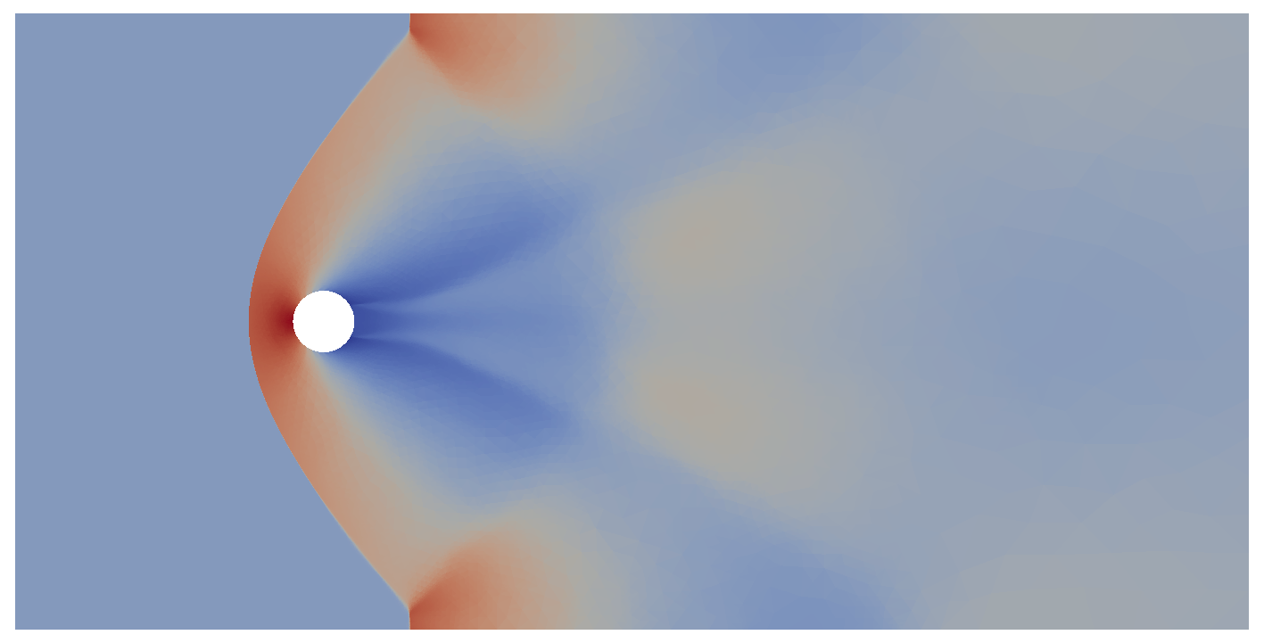Density field shock front capture of a supersonic cylinder modelled by the compressible Euler equations computed using FEniCS and dolfin_dg.

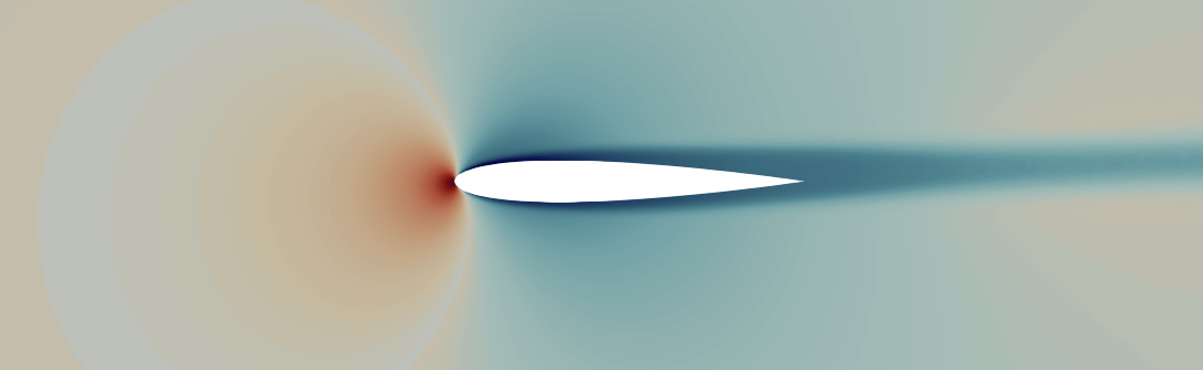Density field of a NACA0012 airfoil modelled by the compressible Navier Stokes system computed using FEniCS and dolfin_dg (Cf. dg_naca0012_2d.py).

Tracer methods & Mantle convection

Tracer methods are widespread in computational geodynamics, particularly for modeling the advection of chemical data. However, they present certain numerical challenges: the necessity for conservation of composition fields and the need for the velocity field to be pointwise divergence free to avoid gaps in tracer coverage. The issues are especially noticed in over long simulation times discretised by many time steps.

The issue of conservation may be addressed by \(l_2\) projection of the tracer data to a FE function whilst constrained by the linear advection PDE. In essence, given \(N_p\) particles each with position \(\vec{x}_p\) and datum \(\phi_p\), composition field \(\phi_h\) and velocity field \(\vec{u}\), at time \(t\) we solve

\[\begin{gather} \min_{\phi_h \in V^h_\text{DG}} \mathcal{J}(\phi_h) = \sum^{N_p}_{p} \frac{1}{2} (\phi_h(\vec{x}_p(t), t) - \phi_p(t))^2, \\ \text{subject to:} \quad \frac{\partial \phi_h}{\partial t} + \vec{u} \cdot \nabla \phi_h = 0. \end{gather}\]

The linear advection equation presents us with the subsequent challenge of mass conservation. Note that

\[\vec{u} \cdot \nabla \phi_h = \nabla \cdot (\vec{u} \phi_h) - \phi_h \nabla \cdot \vec{u}.\]

A velocity field which exactly solves the Stokes system is solenoidal (\(\nabla \cdot \vec{u}\)) and therefore will exactly conserve mass. However, our computed approximations of the velocity \(\vec{u}_h\) may not. We therefore must choose a numerical scheme which exactly satisfies the conservation of mass pointwise such that \(\nabla \cdot \vec{u}_h(\vec{x}) = 0\) for all \(\vec{x}\) in the domain of interest.

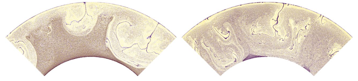Snapshot of a simulation of the Earth’s mantle where tracers track compositional species. The top and base of the domain correspond to the Earth’s surface and the core-mantle boundary, respectively. Left: spurious results encountered in mantle convection where \(\nabla \cdot \vec{u}_h(\vec{x}) \neq 0 \: \forall \vec{x}\). Right: \(\nabla \cdot \vec{u}_h(\vec{x}) = 0 \: \forall \vec{x}\) showing aggregation of material into “piles” at the core-mantle boundary.

Mantle convection simulation. The top slice shows advection of compositional tracers. The lower slice depicts the evolution of the mantle temperature where lighter and darker colours represent hot and cold material, respectively. Note the hot upwellings entraining chemical material to the Earth’s surface, and material sinking from the surface in cold downwellings to be trapped into piles at the core-mantle boundary.

Numerical modeling of subduction zones

Along localized regions of the planet’s surface the Earth’s tectonic plates converge, slamming into each other. Typically one plate, the slab, is driven deep into the Earth underneath the overriding plate. This forms a wedge shaped domain in which the circulation and temperature of the Earth’s mantle is largely controlled by the downgoing slab. These regions are subduction zones and understanding their behavior is key to understanding volcanism and earthquakes around the world.

Numerical modeling of these subduction zones present a number of challenges:

1. Mesh generation from point cloud data obtained from seismological surveys,
2. Contact conditions along a prescribed evolving interface,
3. Local discontinuities in pressure and continuity in velocity,
4. Efficient interpolation between non-matching meshes,
5. Performance of solvers with \(\backsim 10^8\) of degrees of freedom and complicated mesh geometries.

This is investigated in Sime et al. 2023 where we also provide an open source numerical implementation in the respository github.com/nate-sime/mantle-convection.

Rendering of a 3D model loosely approximating the putative evolution of the subduction zone at the Chilean Argentinean border over 11 Myr. Tracers are added where tails show ~1 Myr long pathlines. There is very minor movement in the tracers located in the plate, their displacement is dictated by the slab deformation above the plate depth. See, for example, Sime et al. 2023, Fig. 16.